Contents

Double Pendulum Fractal Map

Author: Tyler Jones Contact: tjjones6@wisc.edu Institution: University of Wisconsin-Madison Date: 05.27.2024

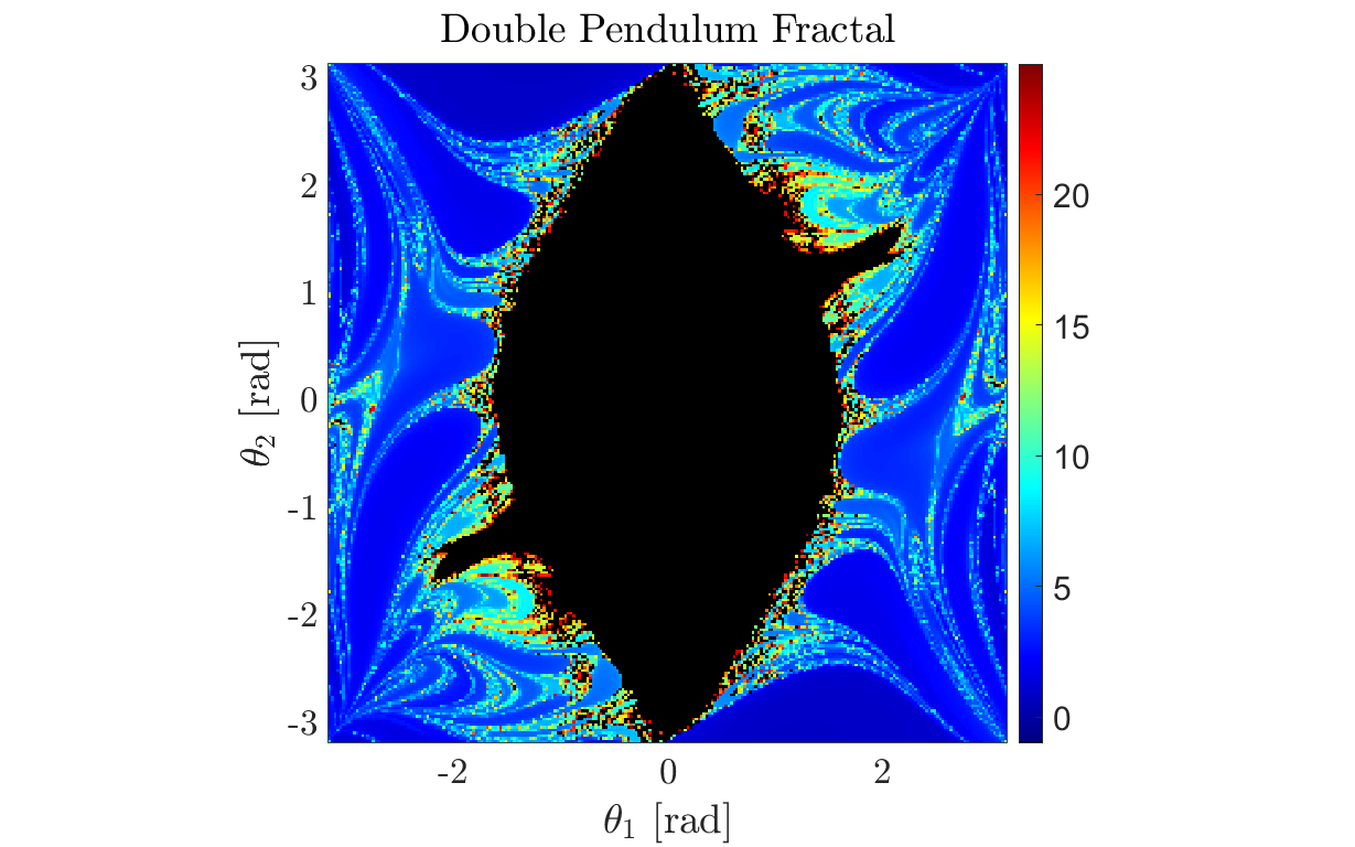
Description: This script simulates a double pendulum system and generates a fractal map that illustrates the behavior of the system for various initial conditions. The simulation uses the ODE45 solver to numerically integrate the equations of motion, capturing the time at which the second pendulum flips. The resulting data is visualized in a heatmap, where each point represents the time of the flip for a specific set of initial angles.

Analysis: https://tjjones6.github.io/DoublePendulum/

close all; clear all; clc;

User Input

g = 9.80665;  % Acceleration due to gravity (m/s^2)
L1 = 1.0;        % Length of the first pendulum arm (m)
L2 = 1.0;        % Length of the second pendulum arm (m)
m1 = 1.0;       % Mass of the first pendulum bob (kg)
m2 = 1.0;       % Mass of the second pendulum bob (kg)

% Initial Conditions
fidelity = 250; % Controls the number of gridpoints
theta1 = linspace(-pi,pi,fidelity);  % Initial angle of the first pendulum (radians)
theta2 = linspace(-pi,pi,fidelity);  % Initial angle of the second pendulum (radians)
omega1_0 = 0;  % Initial angular velocity of the first pendulum (rad/s)
omega2_0 = 0;  % Initial angular velocity of the second pendulum (rad/s)

% Time Span of Simulation
t_final = 25; % (s)
tspan = [0 t_final];

Numerical Integration using ODE45

% Initialize a matrix to store the flip times
flipTimes = NaN(fidelity, fidelity);

% WARNING: Must have the parallel computing toolbox installed. Otherwise
% replace 'parfor' with 'for' loop
tic % Not needed, but keeps track of how long the code runs
parfor i = 1:fidelity

    % Uncomment below if using a simple for loop
    % clc
    % fprintf('Map Completed: %.2f%%\n', i/fidelity*100)

    for j = 1:fidelity
        % Set initial conditions for the current pair of angles
        IC = [theta1(i), omega1_0, theta2(j), omega2_0];

        % Use ODE45 to integrate until the event (flip) occurs
        options = odeset('RelTol', 1e-6, 'AbsTol', 1e-6, 'Events', @stopEvent);
        [~, ~, t_event, ~, ~] = ode45(@(t, y) doublePendulumODE(t, y, g, L1, L2, m1, m2), tspan, IC, options);

        % Store the time of the event (flip) if it occurred
        if ~isempty(t_event)
            flipTimes(i, j) = t_event(1);
        end
    end
end
toc

Elapsed time is 89.751643 seconds.

Plotting Results

% Set NaN values to a specific number outside the range of normal flip times
flipTimesWithNaN = flipTimes;
flipTimesWithNaN(isnan(flipTimes)) = NaN;

% Transpose the data to correct orientation if necessary
flipTimesWithNaN = flipTimesWithNaN';

% Create a custom colormap
cmap = colormap(jet);
cmap = [0 0 0; cmap];  % Add black color for NaN values

% Plotting the fractal map using a heatmap
figure('units','normalized','Position',[0.1 0.1 .8 .8])
myfigpref
hold on; axis tight; axis equal;
imagesc(theta1, theta2, flipTimesWithNaN)
colormap(cmap); colorbar;
clim([-1 max(flipTimes(:))]);  % Set color axis to include the special NaN value
fig_xytit('$\theta_1$ [rad]','$\theta_2$ [rad]','Double Pendulum Fractal')
hold off

Define the function for the double pendulum ODEs

function dydt = doublePendulumODE(~, y, g, L1, L2, m1, m2)
    % Unpack the state variables
    theta1 = y(1);
    omega1 = y(2);
    theta2 = y(3);
    omega2 = y(4);

    % Store equations of motion
    dydt = zeros(4, 1);
    dydt(1) = omega1;
    dydt(2) = (-g * (2 * m1 + m2) * sin(theta1) - m2 * g * sin(theta1 - 2 * theta2) - 2 * sin(theta1 - theta2) * m2 * (omega2^2 * L2 + omega1^2 * L1 * cos(theta1 - theta2))) / (L1 * (2 * m1 + m2 - m2 * cos(2 * theta1 - 2 * theta2)));
    dydt(3) = omega2;
    dydt(4) = (2 * sin(theta1 - theta2) * (omega1^2 * L1 * (m1 + m2) + g * (m1 + m2) * cos(theta1) + omega2^2 * L2 * m2 * cos(theta1 - theta2))) / (L2 * (2 * m1 + m2 - m2 * cos(2 * theta1 - 2 * theta2)));
end

Event function to stop the integration after pendulum flips

function [value, isterminal, direction] = stopEvent(~, y)
    theta2 = y(3);  % Angle of the second pendulum
    value = abs(theta2) - 2*pi;  % Condition for the event
    isterminal = 1;  % Stop the integration
    direction = 0;  % Detect both increasing and decreasing directions
end

Reference Functions for Plotting

% Barrowed from T.G.J. Chandler @UW-Madison Mathematics
function myfigpref
    set(0, 'DefaultAxesFontSize', 20);
    set(0, 'DefaultAxesLineWidth', 2);
    set(0, 'DefaultLineLineWidth', 2);
    set(0, 'DefaultPatchLineWidth', .7);
    set(0, 'DefaultLineMarkerSize', 6);
    grid on;
    box on;
    h = gca;
    h.TickLabelInterpreter='latex';
    h.MinorGridAlpha=0.05;
    h.GridAlpha=0.05;
    h.FontSize=25;
    h.LineWidth=2;
    h = gcf;
    h.Color = [1,1,1];
end

function fig_xytit(xlab, ylab, tit)
    if nargin < 3
        tit = '';
    end
    xlabel(xlab, 'interpreter', 'latex');
    ylabel(ylab, 'interpreter', 'latex');
    title(tit, 'interpreter', 'latex');
end

Published with MATLAB® R2023b